routine + templates makes things easier

With each of the experiments I am running I inflict elevated pressure and temperature on two different tiny gold capsules full of powder. One of them is always full of powder “NM” while the other contains powder “NP”. Even though it is generally possible to tell the two capsules apart before they go into the piston cylinder (by making a sketch of the actual shape of the welded ends, since no two are ever quite the same), the pressure they are subjected to generally means that it is harder to tell them apart when they come out. Fortunately, it is possible to use the microprobe to do a scan over a largish patch of the sample and obtain numbers which are, more or less, representative of the bulk composition of that region.

The first time I did this it felt difficult to compare those numbers with the actual, known, bulk composition of the samples, since this rough-area scan is never going to give precisely the same numbers as the bulk composition. The growth of minerals within the powder has caused some elements to be concentrated in some minerals, and other elements in other minerals. However, in general, the relative differences between the two bulk compositions can still be distinguished via the rough scan. Therefore I set up a spreadsheet with graphs, plotting the original, known, bulk composition in one colour (hollow symbols for NM and solid symbols for NP), and the rough area scans of the first experiment in another. Sure enough just as the original bulk NM is higher in Al₂O₃ and lower in K₂O FeO and CaO than is NP, so the first experiment has one capsule with higher Al₂O₃ and lower FeO, K₂O, and CaO than the other. The second experiment repeated the pattern, but now that I’ve added the third the graph is even easier to read, for now the symbols for the NP bulk plot in one distinct clump on each graph, whilst the ones for the NM bulk composition samples plot in another. This means that from here on out, I need only enter in the new data into the spreadsheet, and in a second’s glance at the chart I’ll know which is which.

Somehow, I really enjoy these tricks which make life easier. Besides, it is fun to set up the charts and graphs.

Two weeks left to finish analyzing the data from my first three experiments and prepare my poster for AGU. Somehow, I suspect that this will keep me as quiet on the blog front as the past couple of weeks when I had both unpacking to do and thesis corrections to make (since my household goods and the examiner’s report arrived on the same day).

blogging at AGU

I've just added my details to the blogroll for the AGU meeting (it should show up tomorrow when they update it) and I plan on attending the geoblogger's Lunch on Wednesday of the conference. I'm looking forward meeting fellow geobloggers there.

Experimental petrology defined

A new friend of mine asked what I do, so I replied that I do research at the university here. He replied "Very Cool ----What is the research in -?" To which I couldn’t help but reply simply “Experimental Petrology”.

However, knowing that the vast majority of the people out there haven’t a clue what that means, I wrote him the following translation:

I am a Geologist who inflicts extreme heat and pressure on tiny amounts of powder (of known composition, which is similar to a specific rock type) for one to three weeks at a time. I then analyze the minerals which grew from the powder to determine which ones are present, and the precise composition of each. Once these experiments have been repeated for a variety of temperatures and pressures (each of which is comparable to specific depths under ground) it is possible to determine which chemical reactions are happening at which temperatures/pressures (for that specific composition). This information is then used (both by myself and by other geologists) to help calculate the temperatures and pressures at which real minerals in real rocks probably grew.

note to self

This note to self isn’t really needed, anymore, having just had to make the change for 27 different figures in 19 CorelDraw documents; I think I will remember forever. However, sometimes it comforts others to hear about my silly mistakes; therefore I’ll say it here publicly:

Photos of thin sections are taken in either crossed-polarized or plane-polarized light. Just because plane polarized light photos tend to be less colourful than crossed-polarized light photos does not make them “plain”.

That’s it. You may now resume your other blog reading. Hope my lesson brought a smile to your face.

Making choices

I have finally received the examiner’s reports from my thesis (submitted back in June). Much to my delight the suggested corrections they have requested are minor, so it shouldn’t be too much longer until the degree is granted.

There was one statement in the examiner’s report which raised my eyebrows a bit. One of the two examiners expressed “surprise” that I made no use of Thermocalc “pseudosections”, which said examiner has found to give consistent results for a variety of compositions. He is correct; my thesis did not make use of that particular program for that task. Instead I used the program Perple_X, to which I was introduced first. I did consider also learning Thermocalc, and Theriak-Domino as well, since each program approaches the task slightly differently. However, it was recommended to me that rather than learning several different programs for the same sort of tasks that I instead focus on one and use the time not spent learning the mechanics of the other programs generating additional data for other aspects of the thesis. Around this same time I read a paper* by an author who did take the time to use those three different programs to model the same samples, and achieved similar, though not identical, results with each. The advice sounding reasonable to me, and the paper further convinced me that since different tools will give similar results that the important thing was to simply choose one of them. I can fully understand having a preference for one program over the other when doing such modeling and creating such diagrams, but never will I be surprised if a student working on their PhD chooses to go with only one program to accomplish a specific type of task. Today’s students are given a limited amount of time to complete their degree and failure to submit the thesis by the University imposed deadline results in loss of funding/support. Given such constraints it is not possible to use every program available, without sacrificing other sections of the research and some choices must be made.

*Hoschek, G., 2004. Comparison of calculated P-T pseudosections for a kyanite eclogite from the Tauern Window, Eastern Alps, Austria. European Journal of Mineralogy, 16(1), 59-72.

first experiment photos

Yesterday I wrote about the effect of water saturation on the size of the crystals grown in my experiments. Today I've got photographs:



These are back-scatter electron images, which means that the brighter the pixel, the heavier elements present at that point (and the darker the pixel, the lighter the element). The bright ring-like objects are rims of iron-rich garnet growing on the seeds of Mg-garnet that was present in the powder before running the experiment. The bright dots of the same tone of brightness as the rings are new Fe-rich garnets growing in the matrix. As you can see, there is a pronounced difference in quantity and size between the two samples. Note the difference in the scale bars between the two photos.

water is important for growth, even for minerals

One of the joys about the learning to run experiments process is that one gets to learn the results of both intended and unintended phenomena. In my experiments the intention is to seal powder of known composition into gold capsules along with a sufficient H₂O and graphite to ensure that the chemical reactions which take place when we elevate the pressure and temperature (to simulate what happens to rocks buried at great depth) take place in “water-saturated” conditions (which is to say there is enough water available for the growth of minerals which require water as part of their chemical formula, such as the micas). However, learning to weld the capsules is a difficult process (I’ve got a draft post on that topic just waiting for me to get photos that actually display the features I want them to show).

As a result of my welding trials and tribulations I’ve had mixed success in the “sealing” part of the above paragraph. Despite the issues with my first attempts at sealing, we ran my first experiment nonetheless, giving two samples a week and a half at elevated pressure/temperature (in this case 650 C and 25 kbars). Once they were “cooked” we had the gold capsules mounted into small disks of epoxy, then carefully polished the disks until the insides of the capsules were exposed. During the polishing stage we received our first confirmation that they had not achieved the same level of “sealed”. Apparently when properly sealed the presence of water inside the capsules ensures that the pore space in between the grains of powder are occupied, and as a result even the high pressures to which we subject them aren’t enough for the new minerals to properly interlock when they grow. As a result, while there are new crystals present, the texture isn’t very rock-like, and when polishing it is easy to accidentally remove clumps of the sample itself. This is the texture we were anticipating, and, for one of the samples run in the first experiment, this is exactly what happened. In these cases we polish only enough to just expose the inside of the capsule, then add more epoxy, letting it soak down into those pore spaces and let it dry before completing the polishing process without so much risk in losing what we are trying to polish.

However, in the other of the two samples run in the first experiment I must not have done the final welding properly, because the contents of the capsule were much harder, and held together better, meaning that the pore space was not held open with fluid when the minerals were growing. This was obvious during the polishing process, so I was able to go quite a bit deeper into the capsule (remember these are only 2 mm in diameter and about 5 mm long so “deeper” is only a relative term) before needing to add the additional epoxy.

Today we got to look at these samples in the microprobe, and as expected from the difference in their textures noted while polishing them, they are rather different from one another. The one wherein I had issues with the welding did contain some water; we know this because there are very small grains of mica present. However, neither was it water-saturated, so it lost some due to the poor seal of the capsule. It contains many, many very tiny grains of garnet (~1 micron diameter; remember that there are 1000 microns in every millimeter) which nucleated on their own, and very thin rims of garnet on the “seeds” which had been included in the powder to encourage garnet growth. The rest of the sample is even finer grained “matrix” minerals, which are going to be difficult to analyze. The other, water saturated, sample contains fewer, larger, grains of garnet, and the rims of new garnet growth on the “seeds” are much thicker than in the first sample. While it, too, is generally fine-grained, it will be easier to find single crystals large enough to get a good analysis of their compositions (which we need if we are going to accomplish our goals).

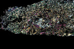
Having had this first look at the samples we’ve set the probe to create “element maps”, pretty full-colour pictures showing which areas are high (warm colours) and which areas are low (cool colours) in specific elements. Once we have these maps, we will use them to select the grains for the detailed compositional analysis. But even before we do that, I now have a better understanding of the difference between water-saturated and water-under saturated environments in terms of the ease at which minerals grow.